

libhedra tutorial notes¶

Introduction¶

libhedra is a library that targets the processing of polygonal and polyhedral meshes, that are not necessarily triangular. It supports the generation, analysis, editing, and optimization of such meshes.

The underlying structure extends the general philosophy of libigl: the library is header only, where each header contains a set of functions closely related. For the most part, one header contains only one function. The data structures are, for the most part, simple matrices in Eigen, and the library avoids complicated and nested structures, relying instead on standalone functions. The visualization is done on the basis of libigl viewer, with some extended options that allow the representation and rendering of polygonal meshes.

The header files contain documentation of the parameters to each function and their required composition; in this tutorial we will mostly tie the functionality of libhedra to the theoretical concepts of polygonal mesh processing and representation.

Installing the tutorial examples¶

This tutorial comprises an exhaustive set of examples that demonstrates the capabilities of libhedra, where every subchapter entails a single concept. The tutorial code can be installed by going into the tutorial folder from the main libhedra folder, and typing the following instructions in a terminal:

mkdir build
cd build
cmake -DCMAKE_BUILD_TYPE=Release ../
make

This will build all tutorial chapters in the build folder. The necessary dependencies will be appended and built automatically. To build in windows, use the cmake-gui .. options instead of the last two commands, and create the project using Visual Studio, with the proper tutorial subchapter as the “startup project”.

To access a single example, say 202_ModelingAffine, go to the build subfolder, and the executable will be there. Command-line arguments are never required; the data is read from the shared folder directly for each example.

Most examples require a modest amount of user interaction; the instructions of what to do are given in the command-line output upon execution.

Polygonal mesh representation¶

libigl represents triangle meshes by a pair of matrices: a matrix V that stores vertex coordinates, and a matrix F that stores oriented triangles as vertex indices into the rows of V. Polygonal meshes are characterized by an arbitrary number of vertices per face (face valence, or degree), and so the mesh representation in libhedra provides an extension of this compact representation with two matrices and a vector:

Eigen::MatrixXd V;
Eigen::VectorXi D;
Eigen::MatrixXi F;

Where V is a #V by 3 coordinates matrix, D is an #F by 1 vector that stores the degree (amount of vertices or edges) in a face, and F is a #F by max(D) array of oriented polygonal faces. In every row of F, i.e. F.row(i), only the first D(i) elements are occupied. The rest are “don’t care” and are usually set to -1 to avoid errors.

This representation has a few advantages:

Triangle meshes are represented the same as in libigl, when one can ignore D (which would then be an array of constant 3), allowing for full compatibility.
Uniform (all faces are with the same valence) meshes are represented compactly.
Avoiding dynamic allocations inside array is memory friendly.
Simple and intuitive indexing.

The disadvantage is when a mesh contains relatively a few high-degree faces accompanied by many low-degree ones. Then, max(D) is high, and a major part of the memory occupied by F is not used. However, this type of meshes are rare in practice.

Mesh Combinatorics¶

While V and F represent the raw information about a polygonal mesh, combinatorial information is often required. It can be obtained with the following function:

#include <hedra/polygonal_edge_topology>

hedra::polygonal_edge_topology(D, F, EV, FE, EF, EFi, FEs,InnerEdges);

where:

Name	Description
`EV`	$2$ elements per row of edge endpoints (into `V`)
`FE`	$max(D)$ consecutive edges per face, where `EV.row(FE(i,j))` contains `F(i,j)` as one of its endpoints.
`EF`	Indices into `F` of the (up to) two adjacent faces per edge.
`EFi`	The relative location of each edge $i$ in faces `EF.row(i)`. That is, `FE(EF(i,0),EFi(i,0))=i` and `FE(EF(i,1),EFi(i,1))=i`. In case of a boundary edge, only the former holds (also for EF).
`FEs`	`FEs(i,j)` holds the sign of edge `FE(i,j)` in face `i`. That is, if the edge is oriented positively or negatively relative to the face.
`innerEdges`	a vector of indices into `EV` of inner (non-boundary) edges.

Chapter 1: I/O and Visualization¶

101 Loading and Visualization¶

Meshes can be loaded from OFF files, which have a similar data structure, with the following function:

polygonal_read_OFF(filename, V, D, F);

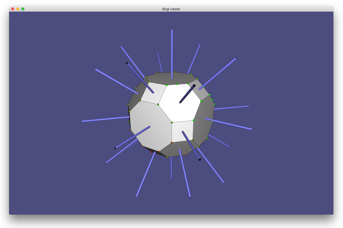
libhedra builds upon libigl viewer for visualization and interaction. libigl viewer currently only supports triangle meshes, and therefore we visualize our meshes by triangulating the faces using hedra::triangulate_mesh. Visualization can be worked out through the following code snippet from examples\visualization:

hedra::polygonal_read_OFF(DATA_PATH "/rhombitruncated_cubeoctahedron.off", V, D, F);
hedra::triangulate_mesh(D, F,T,TF);
hedra::polygonal_edge_topology(D,F, EV,FE, EF, EFi, FEs, innerEdges);
igl::viewer::Viewer viewer;
viewer.data.clear();
viewer.data.set_mesh(V, T);

T is the resulting triangle mesh, and TF is a vector relating every triangle to the face it tesselates. In this manner, one can easily adress the set of triangles belonging to a single face for purposes of visualization (say, a uniform color).

Nevertheless, the default edges in the show overlay feature of the libigl viewer will show the triangulated edges. To see the polygonal edges and nothing else, the following code from examples\visualization can be used:

Eigen::MatrixXd origEdgeColors(EV.rows(),3);
origEdgeColors.col(0)=Eigen::VectorXd::Constant(EV.rows(),0.0);
origEdgeColors.col(1)=Eigen::VectorXd::Constant(EV.rows(),0.0);
origEdgeColors.col(2)=Eigen::VectorXd::Constant(EV.rows(),0.0);
viewer.data.clear();
viewer.data.set_mesh(V, T);
viewer.data.set_edges(V,EV,OrigEdgeColors);

Augmenting the libigl viewer¶

libhedra adds some extra functionality to the libigl viewer with the following functions:

Function	Description
`Scalar2RGB`	Converts a value within $\left[0,1\right]$ into the cool/warm color map ¹[], which can be fed to `igl::set_colors`. Values above or below this range are clamped.
`point_spheres`	Creates spheres with configurable radius, resolution, and color that can be used, e.g., for visualizing deformation handles.
`line_cylinders`	Creates cylinders that can be used to visualize vectors and lines.
`edge_mesh`	Tesselates a mesh by inserting a center point within each face, and creating triangle with each edge. The purpose is to be able to visualize edge-based functions.

line_cylinders and point_spheres create new meshes, and these need to be concatenated to a given mesh in order to be visualized, as the following code (from `examples\visualization’):

hedra::point_spheres(bc, sphereRadius, sphereGreens, 10, false, sphereV, sphereT, sphereTC);
Eigen::MatrixXd bigV(V.rows()+sphereV.rows(),3);
Eigen::MatrixXi bigT(T.rows()+sphereT.rows(),3);
if (sphereV.rows()!=0){
    bigV<<V, sphereV;
    bigT<<T, sphereT+Eigen::MatrixXi::Constant(sphereT.rows(), sphereT.cols(), V.rows());
        bigTC<<TC, sphereTC;
} else{
    bigV<<V;
    bigT<<T;
    bigTC<<TC;
}

viewer.data.clear();
viewer.data.set_mesh(bigV,bigT);

Note: sphereT indices are relative to sphereV, and therefore need to be adjusted to indices in bigV before concatenation.

102 Evaluation¶

libhedra provides functionality to evaluate common properties on meshes. They can be face-, edge-, or vertex- based. The evaluation functions are demonstrated in examples\evaluation

Planarity¶

The planarity of a quadrilateral with vertex positions $q_1,q_2,q_3,q_4$ is often measured by the percentage of the distance between the diagonals $q_3-q_1$ and $q_4-q_2$ to the average diagonal length. Planarity of higher-degree faces is measured as the root-mean-square error of all consecutive quadrilaterlas within the face. That is, for a polygonal face $f=q_1,\cdots,q_d$ , we get:

$$ Planarity(f)=\frac{\sqrt{Planarity(q_1,\cdots,q_4)^{2+\cdots+Planarity(q_{d-2},\cdots,q_1)}2}}{d} $$ The usual reasonable tolerance is 1%. The libhedra function is planarity(V,D, F,p).

Concyclity¶

The concyclity of a quadrilateral with vertex positions $q_1,q_2,q_3,q_4$ measures how much the quad deviates from being concyclic, or \emph{circular}. Consider the two triangles $T_1=q_1,q_2,q_3$ and $T_2=q_3, q_4, q_1$ , and their circumcircles. Then, the concyclity of the quad can be measured as the intersection angle between the (tangents to the) circles at the intersection points $q_1$ and $q_3$ . A rule-of-thumb tolerance is under $5^{\circ}$ . The libhedra function is concyclity(V,D, F,c).

Quaternionic cross-ratios¶

We treat coorrdinates in $\mathbb{R}^3$ as imaginary quaternions in $Im\mathbb{H}$ . That is, with zero real part. Given four coordinates $q_1,q_2,q_3,q_4$ as imaginary quaternions, the quaternionic cross-ratio can be defined in several isomorphic ways. A standard one is:

$cr_{1234}=(q_2-q_1)(q_3-q_2)^{-1}(q_4-q_3)(q_1-q_4)^{-1}.$

The quaternionic cross-ratio encode two interesting geometric properties, that are also Möbius invariant:

The length cross-ratio $\left|cr_{1234}\right|$ , which is the cross ratio of the respective edge lengths.
The phase cross ratio $arg(cr_{1234})$ , that is in fact the circle intersection angle as discussed above.

libhedra provides the following function to compute the cross ratio:

hedra::quat_cross_ratio(V, Q, cr)

where Q is a quadruplet of indices into V, and cr is the result in $\left|Q\right| \times 4$ dimensions, representing a quaternion as $\left(r,\bar{v}\right)$ .

Chapter 2: Polyhedral Mesh Processing¶

201 Planarization¶

TBD

202 Modeling with Affine Maps¶

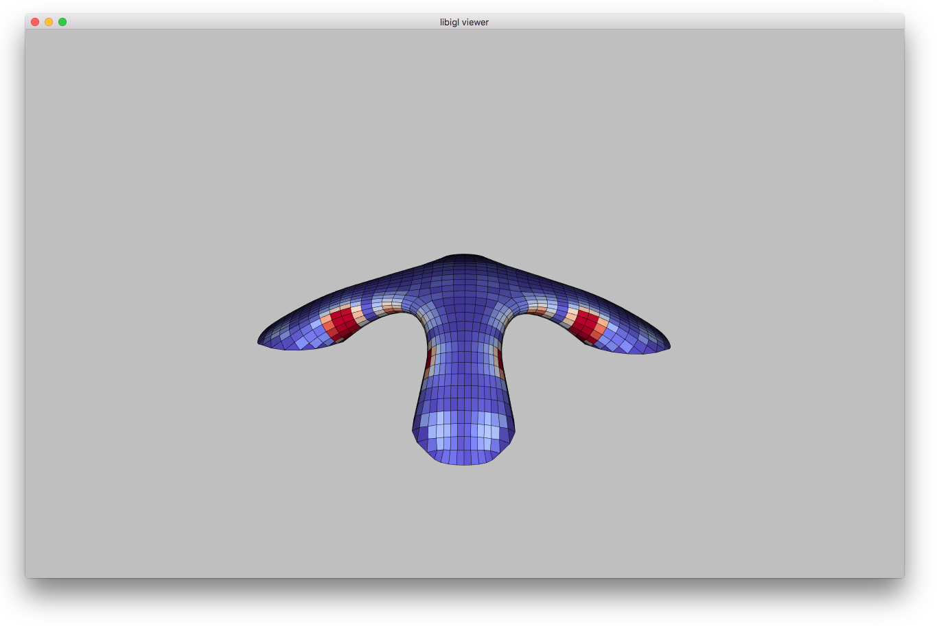
Modelling polyhedral meshes with affine maps was done in ² for the purpose of shape handle-based deformation, interpolation, and shape-space exploration. They use a single affine map per face to preserve planarity. The space of valid space is then linear. libhedra implements the deformation algorithm according the version detailed in the auxiliary note. The algorithm is demonstrated in examples\modeling_affine.

The algorithm operates in two stages: a precompute stage that takes into account the original geometry and the handles, and a deformation stage, that takes into account the user prescription of handle positions. The precompute stage is the most computationally-expensive, as it factorizes the involved matrices, but it only has to be called once per choice of deformation handles.

The functions are then:

#include <hedra/affine_maps_deform.h>

affine_maps_precompute(V,D, F,EV,EF,EFi, FE,h,alpha, beta, adata)
affine_maps_deform(adata, qh, numIterations, q)

where (parameters (e.g., EF) that have been discussed before with the same name have the same description):

parameter	Description
`h`	A list of handle indices into `V`
`alpha, beta`	Parameters controlling face map prescription vs. map smoothness (see the auxiliary note)
`adata`	A struct of type hedra::affine_data computed by `affine_maps_precompute` and passed to `affine_maps_deform`. Not supposed to be edited by the user.
`qh`	A list of size $\left
`numIterations`	Of the algorithm. Generally referring to the as-rigid-as-possible part of the map prescription.
`q`	The full result in $\left

Optimization¶

Optimization is done in libhedra by generic classes, taking templated trait classes as input. While this is a more complicated design pattern than simple functions, it does provide an elegant way to plug in linear solvers, objectives, and constraints quite easily.

Nonlinear Least Squares¶

Note: the demo currently uses a more sophisticated levenberg_marquadt solver with LMSolver instead of GNSolver below. The user interface is otherwise the same, but the solution algorithm is a somewhat different. The text berlow will be updated soon.

libhedra support nonlinear least squares optimization by Gauss-Newton iterations through the class GNSolver<LinearSolver, SolverTraits> in the respective header file. This class accepts two traits classes: for linear solving, and for the least-squares objectives.

The optimizer solves problems of the form:

$$ x = argmin\sum ^m _{i=0}{(E_i(x))^2}, $$ by taking iterations, each solving the following linear problem:

$J^TJd = -J^tE.$

$E=\left( E_1(x), E_2(x), \cdots E_m(x)\right)^T$ is a column vector of size $m$ decribing the energy at iteration $k$ , and $J=\left(\nabla E_m, \cdots, \nabla E_m\right)^T$ is the (sparse) $m \times n$ Jacobian matrix at that iteration, where $n$ is the size of the solution $x$ . Then, the variable $x^{k+1}$ is updated as follows:

$x^{k+1}=x^k+hd.$

The step size $h$ is determined to be such that does not increase the energy. For this, we begin with a value of $h=1$ , and reduce it by half until it reaches a tolerance value hTolerance.

The initial solution $x_0$ is acquired from the SolverTraits instance (see below).

The algorithm stops when:

$max(|x^{k+1}-x^{k}|) < xTolerance$ (step size) and
$max(|J^T E|) < fooTolerance$ (first-order optimality) or
$h < hTolerance$ .

Initializing the solver is done by calling the GNSolver::init() function once per problem setting. That means whenever the energy computation and Jacobian structures remain the same.

void init(LinearSolver* _LS,
          SolverTraits* _ST,
          int _maxIterations=100,
          double _xTolerance=10e-6,
          double _hTolerance=10e-9,
          double _fooTolerance=10e7).

Solving is done by simply calling GNSOLver::solver(bool verbose). The initial solution will be taken from SolverTraits (see below). verbose indicates a printout of the process of the optimization.

Note that the first-order optimality condition is by default pretty relaxed (or rather mostly disabled).

The trait classes¶

Any LinearSolver class must include the following functionality:

class LinearSolver{
...
bool analyze(const Eigen::VectorXi& _rows,
                         const Eigen::VectorXi& _cols){...}
bool factorize(const Eigen::VectorXd& values){...}
bool solve(const Eigen::MatrixXd& rhs,Eigen::VectorXd& x){...}
...
};

This functionality pertains to symbolic analysis, factorization, and solution of the system. The class should be able to handle the positive semi-definite system of $J^TJ$ that is solved in each iteration of the Gauss-Newton solver, and the analysis function is then only called once per optimization, since the structure of the Jacobian is not supposed to change.

For comfort, a class EigenSolverWrapper<class EigenSparseSolver> that wraps the sparse linear solvers in Eigen is provided. For instance, EigenSolverWrapper<Eigen::SimplicialLDLt> is a good choice.

Any SolverTraits class must include the following functionality:

class SolverTraits{
...
    Eigen::VectorXi JRows, JCols;  
    Eigen::VectorXd JVals;         
    int xSize;                      
    Eigen::VectorXd EVec;         
...
    void initial_solution(Eigen::VectorXd& x0){...}
    void pre_iteration(const Eigen::VectorXd& prevx){...}
    bool post_iteration(const Eigen::VectorXd& x){...}
    void update_energy(const Eigen::VectorXd& x){...}
    void update_jacobian(const Eigen::VectorXd& x){...}
    bool post_optimization(const Eigen::VectorXd& x){...}
...

The functions are callbacks that will be triggered by the optimizer GNSolver, where:

Class Member	Description
`JRows, JCols, JVals`	(row, column, value) triplets in the Jacobian. the (row, column) pairs are expected to stay constant throughout the optimization.
`xSize`	The size of the solution vector `x`.
`EVec`	The vector $E$ of summands in the least squares.
`initial_solution()`	Called before the beginning of the iterations, and needs to provide an initial solution $x_0$ to the solver.
`pre_iteration()`	Called before an iteration with the previous solution.
`post_iteration()`	Called after an iteration with the acquired solution. If it returns `true`, the optimization stops after this iteration. As such, returning `false` wuold allow the solver to convergence “naturally”.
`update_energy()`	Called to update the energy vector `EVec`. It is a staple function that is called quite often, so it should be efficient.
`update_jacobian()`	Called to update the Jacobian values vector `JVals`. It is called at least once per iteration.
`post_optimization()`	Called with the final result after the optimization ended. `post_optimization()` should return `true` if the optimization should cease. Otherwise, it would begin again. This callback possibility is good for when the optimization process requires several consequent full unconstrained optimization processes, for instance, in the Augmented Lagrangian method.

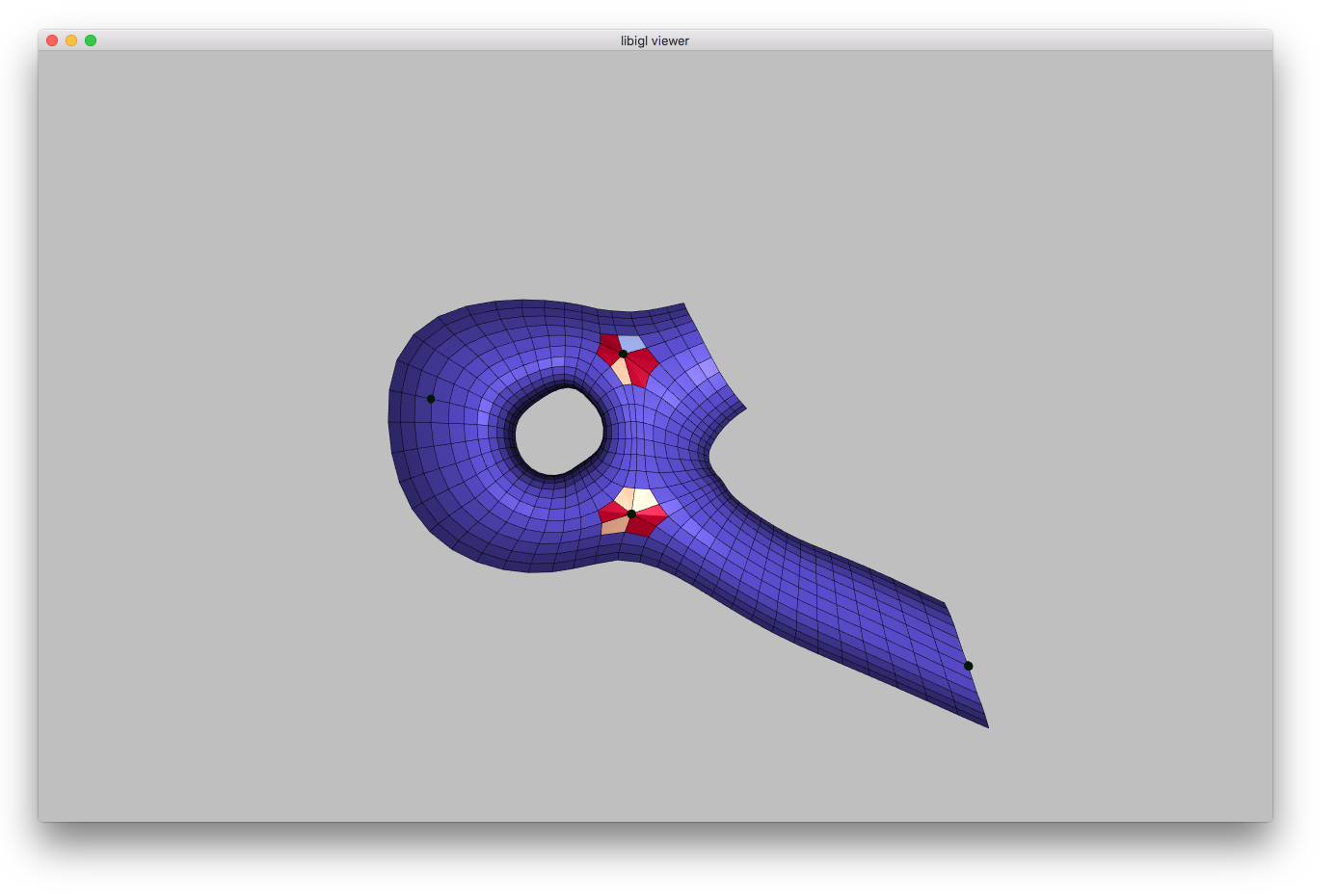
An example of Nonlinear least-squares is done in examples/gauss-newton, implementing a handle-based deformation algorithm, minimizing the length and dihedral angle deviations (similar to ³), and with an initial solution based on biharmonic deformation fields in libigl.

203 Polyhedral Patterns¶

TBD

Chapter 3: Möbius Geometry Processing¶

301 Complex PCM deformation¶

TBD

302 Complex PCM interpolation¶

TBD

303 Quaternionic PCM deformation¶

TBD

304 Regular meshes¶

TBD

Chapter 4: Subdivision Meshes¶

401 Polygonal subdivision¶

TBD

402 Canonical Möbius subdivision¶

TBD

Future Plans¶

The following functionality will soon be available in libhedra:

Parallel and offset meshes, including evaluation of the Steiner formula for discrete curvature.
Local-global iterations for shape projection.
Constrained optimization using augmented Lagrangians.
Polyhedral patterns parametrization and optimization.

If you would like to suggest further topics, would like to collaborate in implementation, complain about bugs or ask questions, please address [Amir Vaxman] (avaxman@gmail.com) (or open an issue in the repository)

Acknowledge libhedra¶

If you use libhedra in your academic projects, please cite the implemented papers appropriately. To cite the library in general, you could use this BibTeX entry:

@misc{libhedra,
  title = {{libhedra}: geometric processing and optimization of polygonal meshes,
  author = {Amir Vaxman and others},
  note = {https://github.com/avaxman/libhedra},
  year = {2016},
}

Kenneth Moreland. Diverging Color Maps for Scientific Visualization. ↩
Amir Vaxman. Modeling Polyhedral Meshes with Affine Maps , 2012 ↩
Fröhlich, Stefan and Botsch, Mario, Example-Driven Deformations Based on Discrete Shells, 2011. ↩